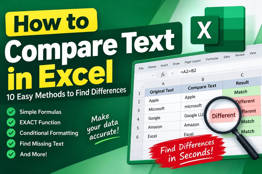
Comparing text in Excel is a useful skill when working with spreadsheets, customer records, product descriptions, employee lists, or large datasets. Even a small difference between two cells, such as an extra space, missing character, or spelling mistake, can cause problems with data accuracy.
Fortunately, Microsoft Excel provides several ways to compare text without manually checking every cell. You can use simple formulas, the EXACT function, conditional formatting, and lookup functions to identify matches and differences quickly.
For example, imagine you have two columns containing customer names. You want to determine whether the names match, identify missing entries, and highlight inconsistencies. Instead of reviewing hundreds of rows individually, Excel can perform these comparisons automatically.
In this guide, you will learn how to compare text in Excel using 10 practical methods, with step-by-step instructions, formulas, examples, and troubleshooting tips.
Whether you are comparing two cells, entire columns, or text from different worksheets, these techniques will help you find differences and improve spreadsheet accuracy.
Why Would You Need to Compare Text in Excel?
Text comparison helps identify inconsistencies between datasets. It is particularly useful when information comes from different sources or when multiple people edit the same spreadsheet.
Common situations include:
- Customer databases: Check whether customer names, email addresses, and contact information match.
- Product inventories: Identify changes in product titles, descriptions, or identification codes.
- Employee records: Compare names, departments, and other information between two reports.
- Content management: Find differences between old and updated text.
- Data cleaning: Detect extra spaces, spelling mistakes, and inconsistent capitalization.
- Report verification: Confirm that information has not changed between spreadsheet versions.
The best comparison method depends on whether you need to compare individual cells, entire columns, or similar-looking text.
How to Prepare Your Excel Data for Text Comparison
Before comparing text, organize your spreadsheet to make the process easier.
For example, suppose you have two columns:
| Column A: Original Text | Column B: Updated Text |
|---|---|
| Apple | Apple |
| Microsoft | microsoft |
| Google LLC | |
| Amazon | Amazon |
Column A contains the original text, while Column B contains the updated information.
You can use Column C to display the comparison results.
For the examples below, assume that your data begins in row 2 and row 1 contains column headings.
If your spreadsheet contains thousands of entries, ensure the correct records are aligned before comparing individual rows. Sorting two lists independently can produce misleading comparisons when entries appear in different orders.
Method 1: Compare Two Text Cells Using the Equal Sign (=)
The simplest way to compare text in Excel is to use the equal sign.
This method checks whether two cell values match and returns either TRUE or FALSE.
Step-by-step instructions
- Open your Excel spreadsheet.
- Enter your original text in cell A2.
- Enter the text you want to compare in cell B2.
- Select cell C2.
- Enter the following formula:
=A2=B26. Press Enter.
Excel will display one of two results:
- TRUE: The cell values match.
- FALSE: The cell values are different.
Example
| Cell A | Cell B | Result |
|---|---|---|
| Apple | Apple | TRUE |
| Microsoft | FALSE | |
| Excel | excel | TRUE |
Important: Excel’s standard text equality comparison is case-insensitive. It treats “Excel” and “excel” as matching values.
However, differences involving extra spaces can cause the comparison to return FALSE.
Best for: Quickly checking whether two text cells contain matching values when capitalization is unimportant.
Method 2: Compare Text Using the IF Function
The IF function is useful when you want descriptive results instead of TRUE or FALSE.
For example, you may prefer Excel to display “Match” when two cells contain the same text and “Different” when they do not.
How to use the IF formula
Select cell C2 and enter:
=IF(A2=B2,"Match","Different")Press Enter and copy the formula down to the remaining rows.
Example results
| Original Text | Updated Text | Result |
|---|---|---|
| WordPress | WordPress | Match |
| Shopify | shopify | Match |
| Microsoft | Different | |
| Excel | Excel Online | Different |
The formula contains three components:
A2=B2checks whether the values match."Match"appears when the condition is TRUE."Different"appears when the condition is FALSE.
You can customize the messages to display “Same,” “Changed,” “Correct,” or “Incorrect.”
For example:
=IF(A2=B2,"No Changes","Text Changed")This is especially useful for comparing product information, employee records, or updated spreadsheet content.
Best for: Creating clear comparison reports that other users can understand without interpreting Boolean results.
Method 3: Compare Text with the EXACT Function (Case-Sensitive)
Sometimes, capitalization matters.
For example, you might need to compare product codes, usernames, or identifiers where uppercase and lowercase letters must be distinguished.
The EXACT function performs a case-sensitive text comparison.
According to Microsoft’s documentation, EXACT checks whether two text strings are identical while ignoring cell formatting differences.
Formula
=EXACT(A2,B2)Example
| Text A | Text B | Result |
|---|---|---|
| Apple | Apple | TRUE |
| Apple | apple | FALSE |
| EXCEL | Excel | FALSE |
| Data | Data | TRUE |
Unlike the regular equal-sign comparison, EXACT recognizes differences in capitalization.
It also detects differences in spaces and other text characters.
Display custom results with EXACT and IF
You can combine both functions:
=IF(EXACT(A2,B2),"Exact Match","Different")This formula returns “Exact Match” only when the two text strings are identical.
For example, if A2 contains “WordPress” and B2 contains “wordpress,” the result will be “Different.”
Best for: Checking capitalization, validating text identifiers, and comparing strings where every character matters.
Method 4: Compare Text While Ignoring Extra Spaces
Two cells may look identical but still produce a FALSE result because one contains additional spaces.
Consider these values:
- A2: “Microsoft”
- B2: ” Microsoft “
The second value contains spaces before and after the word.
A regular comparison identifies them as different.
You can use the TRIM function to remove unnecessary standard spaces before comparing the values.
Formula
=TRIM(A2)=TRIM(B2)This compares the cleaned text.
For a more readable result, use:
=IF(TRIM(A2)=TRIM(B2),"Match","Different")The TRIM function removes leading and trailing standard spaces and reduces consecutive standard spaces between words to single spaces. It does not remove nonbreaking spaces by itself.
Remove invisible characters
If your text was copied from websites, PDFs, or external applications, consider combining TRIM with CLEAN:
=IF(TRIM(CLEAN(A2))=TRIM(CLEAN(B2)),"Match","Different")CLEAN removes certain nonprinting characters, while TRIM handles ordinary spacing.
For nonbreaking spaces commonly found in copied web content, you can use:
=TRIM(SUBSTITUTE(A2,CHAR(160)," "))Apply the same cleaning formula to both values before comparing them.
Best for: Comparing imported datasets, customer lists, and text copied from external sources.
Method 5: Find Text Differences Using the LEN Function
The LEN function counts the number of characters in a cell, including spaces.
It can help diagnose text differences that are difficult to see.
For example:
| Original Text | Updated Text | Length A | Length B |
|---|---|---|---|
| Excel | Excel | 5 | 5 |
| Google LLC | 6 | 10 | |
| Apple | Apple with trailing space | 5 | 6 |
In the final row, the second value is assumed to contain an invisible trailing space rather than the descriptive text shown in the table.
Compare the text lengths
Enter:
=LEN(A2)=LEN(B2)If both text strings have the same length, Excel returns TRUE.
To calculate the difference in character counts:
=LEN(B2)-LEN(A2)A result of 3 indicates that the second cell contains three more characters than the first.
However, equal character counts do not guarantee identical text.
For example, “Apple” and “Grape” have the same number of characters but contain different letters.
Use LEN as a troubleshooting tool alongside EXACT or other comparison formulas.
Best for: Detecting added characters, missing letters, invisible spaces, and unexpected changes in text length.
Method 6: Highlight Text Differences Using Conditional Formatting
Conditional formatting allows you to identify text differences visually without creating an additional results column.
Instead of displaying TRUE or FALSE, Excel highlights cells that meet your comparison condition.
Microsoft supports custom conditional formatting rules that use formulas returning TRUE or FALSE.
Step-by-step instructions
- Open your spreadsheet.
- Select the range
B2:B100. - Navigate to Home → Conditional Formatting.
- Choose New Rule.
- Select “Use a formula to determine which cells to format.”
- Enter this formula:
=$A2<>$B2- Click Format.
- Select a fill color, such as light red.
- Click OK to apply the rule.
Excel will highlight cells in Column B that differ from the corresponding cells in Column A.
The <> operator means “not equal to.”
For example, if A2 contains “Apple” and B2 contains “Orange,” B2 will be highlighted.
Highlight differences with case sensitivity
If capitalization matters, use:
=NOT(EXACT($A2,$B2))This rule also highlights differences such as “Google” versus “google.”
If you want to highlight both comparison columns, select A2:B100 before creating the rule and use the same formula.
Best for: Visually reviewing spreadsheet changes, identifying inconsistencies, and comparing large datasets.
Method 7: Compare Two Columns and Find Missing Text Using COUNTIF
Comparing entire columns is different from comparing two cells in the same row.
Suppose Column A contains customer names from January and Column B contains names from February.
The names may appear in different orders.
A row-by-row comparison would produce incorrect conclusions about whether customers are present in both lists.
The COUNTIF function offers a practical solution.
Formula to find missing entries
Enter this formula in C2:
=IF(COUNTIF($B$2:$B$100,A2)>0,"Found","Missing")The formula searches Column B for the text in A2.
If Excel finds at least one match, the result is “Found.”
Otherwise, the result is “Missing.”
Example
| January List | February List | Result for January |
|---|---|---|
| Apple | Found | |
| Microsoft | Found | |
| Microsoft | Apple | Found |
| Amazon | Netflix | Missing |
Amazon is missing from the February list, even though the other items appear in different rows.
Find items missing from Column A
Reverse the comparison:
=IF(COUNTIF($A$2:$A$100,B2)>0,"Found","Missing")COUNTIF is not case-sensitive. It also supports wildcard matching, so text containing literal asterisks or question marks may need additional handling.
This approach checks whether an item exists at least once. If duplicate counts matter, compare the number of occurrences separately.
Best for: Finding missing customer names, comparing inventory lists, and identifying entries present in one dataset but not another.
Method 8: Compare Text Using XLOOKUP
When two datasets contain unique IDs but their rows are arranged differently, XLOOKUP can find the corresponding record before comparing its text.
Suppose your spreadsheet contains:
- Column A: Original product IDs
- Column B: Original product names
- Column D: Updated product IDs
- Column E: Updated product names
Enter the following formula in C2:
=IFNA(IF(B2=XLOOKUP(A2,$D$2:$D$100,$E$2:$E$100),"Match","Different"),"ID not found")This formula finds the product ID in Column D, retrieves its corresponding name from Column E, and compares that name with Column B.
It returns “Match,” “Different,” or “ID not found.”
This is useful when comparing data that has been reordered. XLOOKUP uses exact matching by default, but it is unavailable in Excel 2016 and Excel 2019.
Best for: Comparing customer records, product databases, and updated reports using unique identifiers.
Method 9: Compare Text Between Two Excel Worksheets
You can compare text stored on different worksheets within the same Excel workbook.
For example, suppose your workbook contains two sheets named Sheet1 and Sheet2.
Create a third worksheet called Comparison.
In cell A2 of the Comparison sheet, enter:
=IF(Sheet1!A2=Sheet2!A2,"Match","Different")The formula compares cell A2 from both worksheets.
Copy it across or down to compare additional cells.
For case-sensitive comparisons, use:
=IF(EXACT(Sheet1!A2,Sheet2!A2),"Match","Different")If a worksheet name contains spaces, surround its name with single quotation marks:
=IF('Old Data'!A2='New Data'!A2,"Match","Different")You can also open both worksheets side by side using View → New Window → View Side by Side for manual inspection.
Best for: Comparing monthly reports, spreadsheet versions, and information stored in separate worksheets.
Method 10: Compare Similar Text Using Power Query Fuzzy Matching
Sometimes, two text values are similar but not identical.
For example:
- “Microsoft Corporation” and “Microsoft Corp”
- “John Smith” and “Jon Smith”
- “International Business” and “International Businesses”
Traditional Excel comparison formulas will generally identify these strings as different.
Power Query provides fuzzy matching to find similar text values.
How to use fuzzy matching
- Convert both datasets into Excel tables using Ctrl + T.
- Select one table and navigate to Data → From Table/Range.
- Create a query for each table.
- Open the Power Query Editor.
- Select Home → Merge Queries.
- Choose the second table and select the text columns to compare.
- Enable “Use fuzzy matching to perform the merge.”
- Adjust the similarity threshold.
- Confirm the merge and load your results into Excel.
Microsoft documents fuzzy matching for Power Query in Excel for Microsoft 365. Its default similarity threshold is 0.80, and you can adjust it according to your requirements.
Fuzzy matching identifies likely similarities rather than guaranteeing that two records refer to the same person or item. Review the results before automatically merging important records.
Best for: Matching inconsistent customer names, handling spelling variations, and comparing large datasets with imperfect text.
Which Excel Text Comparison Method Should You Use?
| Your goal | Recommended method |
|---|---|
| Compare two individual cells | Equal sign |
| Display Match or Different | IF |
| Compare uppercase and lowercase | EXACT |
| Ignore unnecessary spaces | TRIM |
| Detect character count differences | LEN |
| Highlight changed cells | Conditional Formatting |
| Find missing list entries | COUNTIF |
| Match records using IDs | XLOOKUP |
| Compare different worksheets | Cross-sheet formulas |
| Find similar text | Power Query |
Choose your method based on the structure of your data and the accuracy required.
Common Problems When Comparing Text in Excel
Even when formulas are correct, comparisons can produce unexpected results.
1. Identical-looking text returns FALSE
The cells may contain invisible spaces or nonprinting characters. Use TRIM, CLEAN, or LEN to investigate.
2. Different capitalization returns TRUE
Standard equality comparisons ignore capitalization. Use EXACT when capitalization matters.
3. Text comparison produces incorrect matches
Check whether your rows represent the same records. Use unique IDs and XLOOKUP when records appear in different orders.
4. A formula produces an error
Check the cell references, formula syntax, and supported Excel version. Some regional Excel settings use semicolons instead of commas as formula argument separators.
5. Long paragraphs are difficult to compare
Excel can determine whether two paragraphs match, but its basic formulas do not provide a convenient, built-in word-by-word difference view.
For comparing longer paragraphs, documents, or copied website content, a dedicated online text comparison tool can provide a more readable workflow. You can copy text from Excel and compare the two versions using a tool such as TextComparely.
Frequently Asked Questions
1. How do I compare two text cells in Excel?
Use the formula =A2=B2. It returns TRUE when both cells match and FALSE when their values differ. Use EXACT for case-sensitive comparisons.
2. How do I highlight differences between two columns in Excel?
Select the cells in Column B, create a conditional formatting rule, and enter =$A2<>$B2. Choose a fill color to highlight the differences.
3. How can I compare text in Excel without considering case?
Use the equal-sign formula or IF function. For example, =IF(A2=B2,"Match","Different") treats uppercase and lowercase versions of the same text as equal.
4. Can Excel compare two columns and find missing values?
Yes. Use COUNTIF to check whether each value in one column exists in the other. This works even when the items are arranged in different orders.
5. How do I compare two Excel files?
Open both files and use View Side by Side for visual comparison. You can also create formulas that reference cells in both workbooks. Supported enterprise editions include a separate Spreadsheet Compare application for more detailed workbook comparisons.
6. Can Excel identify individual word differences in paragraphs?
Basic Excel formulas can identify whether paragraphs match, but they do not automatically highlight every changed word within a cell. A specialized text comparison tool is generally more convenient for this purpose.
Conclusion
Learning how to compare text in Excel can save considerable time when reviewing spreadsheets, identifying errors, or validating data.
For simple comparisons, use the equal sign or IF function. Choose EXACT when capitalization matters, conditional formatting when you want to highlight differences, and COUNTIF when comparing entire lists.
For more complex datasets, XLOOKUP and Power Query provide additional ways to match records and identify similarities.
By selecting the appropriate method and cleaning your data before comparison, you can identify text differences more efficiently and maintain more accurate spreadsheets.